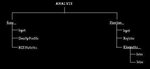
Fig 12.1: Commands under ANALYZE.
Fig 12.1: Commands under ANALYZE.
The main purpose of ANALYZE commands is to allow the analysis of both
scene and structure data so as to quantify specific information relating
to the objects that are imaged. Commands under Scene operate on scenes
and output a variety of quantitative information and those under
Structure operate on structures and structure systems and output
appropriate structure-related quantitative information as well as new
structure systems and structure plans.
12.1 Scene
12.1.1 Summary of Commands
These commands allow analyzing scenes in a slice-by-slice fashion to
extract certain quantitative information based on cell intensities.
Input allows selecting files of type IM0.
Density Profile can be used to specify paths within the scene domain
along which cell density distribution can be computed and displayed as a
graph. These graphs can be output for later usage. ROIStatistics allows
specifying regions-of-interest within the scene domain and computing
cell intensity statistics within these regions. The statistics can also
be output to a file for later usage or as a record.
12.1.2 Common Options
The common options for commands under Analyze-Scene are: PREVIOUS, NEXT,
SET INDEX, GREYMAP, LAYOUT, and ROI. Among these, PREVIOUS, NEXT, SET
INDEX, and GREYMAP, are described in Section 7.2. LAYOUT and ROI are
short versions of the commands Layout and ROI under
VISUALIZE-Slice-Cycle. These two options have further suboptions as
illustrated in Figure 12.2. These options have been described in Section
7.2.
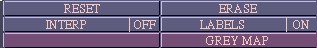
Fig 12.2: Panel Options for LAYOUT and ROI.
The mouse button state diagram associated with LAYOUT and ROI are
similar to those associated with the commands Layout and ROI under
VISUALIZE-Slice-Cycle.
12.1.3 Commands
12.1.3.1 Scene-Input
This command should be used for selecting the desired IM0 file. If the
most recently selected file is appropriate, it is not necessary to
initiate this command. For details of operation, see Section 7.1. Only
one input file is permitted for DensityProfile.
12.1.3.2 Scene-DensityProfile
The main purpose of this command is to make it possible to compute and
display the distribution of cell density along paths specified
interactively by the user. A secondary purpose is to enable the user to
measure widths of structures (such as for vessels, lumens, foramina, and
walls) by indicating points on the profile (say, of greatest slope) that
might represent the structure boundary along the specified path. The
displayed profiles can be saved in user-specified files for later usage,
such as for printing the profile on paper using standard Unix commands.
The mouse-button state diagram associated with this command is shown in Figure 12.3.
Upon selection of DensityProfile, a default slice (usually the slice with all indexes equal to 1) is displayed at a default grey map setting and at a default magnification. The indexes of the slice are displayed at the upper-left corner of the displayed picture as (i_n, . . . . ,i_1), where i_1, . . . . , i_n are the first to nth indexes of the slice in the n-dimensional scene. The scale factor is displayed underneath the indexes as sf = x. The number indicates the magnification factor of the input slice (sf = 2 means that a pixel in the input slice corresponds to two pixels in the displayed picture). The mouse buttons are set to state 1 in Figure 12.3. The figure illustrates how to proceed to specify a path, to display the profile and to measure structure widths based on density distributions.
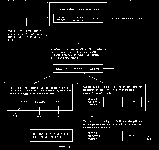
Fig 12.3: Mouse Button State Diagram for DensityProfile. An arrow leaving a
button indicates that that button is clicked.
The panel options available for this command are shown in Figure 12.4. Note that, in state 1 of Figure 12.3, it is not necessary to select successive points on the same slice. For a 3D or 4D input scene, you may change the displayed slice using any of the panel options PREVIOUS, NEXT, or SET INDEX and continue selecting the points to specify the path. For a 3D or 4D scene, a dynamic mode can be selected via the panel option MODE (see below) for specifying a path along which only time changes. In this mode, you cannot select more than one point on the same slice for the same path. In states 4 and 5, the points to indicate where the structure boundary may lie along the path should be selected within the display area of the profile.
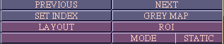
Fig 12.4: Panel Options for DensityProfile.
MODE: This is a switch with two states called STATIC (default sate) and DYNAMIC. In STATIC state, there are no restrictions on how the points are selected to indicate the path for density profile computation. For a 3D scene, this means that you can specify essentially any path in the 3D space of the scene domain. By choosing the path to be approximately perpendicular to an aspect of an object represented in the scene, the profile of cell density across this aspect can be computed and displayed. Further, by selecting two points, one in the ascending part of the profile and the other in the descending part, the width of this aspect can be measured. In STATIC state, for a 4D scene, care should be exercised in specifying the path. If the 4D scene represents a dynamic object such as the heart (with the fourth dimension being time), arbitrary paths in the 4D spatio-temporal space may not have any meaning. If an object point (such as an anatomic landmark on the heart) can be tracked and indicated for successive time instants, the path so indicated essentially corresponds to purely change of time. Hence, the resulting profile corresponds to a time density curve of the object point. In DYNAMIC sate of the switch MODE, you are forced to select only one point on the same slice. Therefore, this mode is more convenient for studying time density profile of dynamic phenomena.
The remaining panel options work as descried in Sections 7.2 and 12.1.2.
The static option SAVE in the mouse window (see Section 7.3) can be used
to save the current density profile in a file whose name appears in the
tablet associated with the SAVE option. You may change this name as
described in Section 7.3. The profile saved in this file can be later
displayed using the Unix command gnuplot
The mouse button state diagram associated with this command is shown in
Figure 12.5.
Upon selection of ROIStatistics, a default slice (usually the slice with
all slice indexes equal to 1) is displayed at a default grey map setting
and at a default magnification. The indexes of the slice are displayed
at the upper-left corner of the displayed picture as
(i_n, . . . . , i_1), where i_1, . . . . , i_n are the first to nth
indexes of the slice in the n-dimensional scene. The scale factor is
displayed underneath the indexes as sf = x. This number indicates the
magnification factor of the input slice (sf = 2 means that a pixel in
the input slice corresponds to two pixels in the displayed picture). The
mouse buttons are set to state 1 in Figure 12.5 and the user should
proceed as illustrated in this figure to measure roi statistics. Figure
12.5(a) shows how statistics can be measured for user-drawn regions and
Figure 12.5(b) shows how statistics can be measured for rois of
predetermined size.
In the table, the slice indexes are listed under "slice#" and the type
of roi ("free", 55", etc.) under roi. For 2D roi's, the figure in the
last column represents area of the roi. For 3D, this number represents
the volume of the roi. The last row, Total, indicates the total (or
overall) statistics. For min, max, mean, and std.dev, this corresponds
to the min, max, mean and std.dev considering all roi's that are listed.
The entry under Area/Volume in the row Total represents sum of
areas/volumes of all roi's that are listed. While in state 3 in Figure
12.5, the user can scroll the listing in the table up or down by
clicking (with left/middle mouse button) on the scroll buttons in the
table.
The panel options associated with ROIStatistics are shown in Figure
12.7.
TYPE: This is a switch with seven states, called FREE, 55, 555, 77, 777,
99, and 999. In state FREE, the user is allowed to specify free-form roi
by drawing a closed curve. The operations associated with this state are
illustrated in Figure 12.5(a). In the remaining states, the roi's are of
rectangular shape. The size indicated by the state, for example 55,
means that the roi is of that size in the original slice. In the
displayed picture, the size may be larger or smaller depending on the
scale factor.
GRAD: This is a switch with two states, called 2D and 3D. In state 2D, a
2D gradient operator is used to compute gradient-related statistics. In
state 3D, a 3D operator is used for this purpose. In some situations,
the 3D operator may give more accurate results if you are dealing with
3D or 4D scenes.
The static option SAVE in the mouse window (see Section 7.3) can be used
to save the roi statistics currently listed in the table in a file whose
name appears in the tablet associated with the SAVE option. You may
change this name as described in Section 7.3. The information saved in
this file can be recalled in a future session with ROIStatistics by
simply changing the file name to the name of the saved file.
Input allows selecting appropriate input files. Both Register and
Kinematics expect input to be binary shells of type Shell1. Hence, the
appropriate input files are BS1 files or PLN files that contain Shell1
structures. Register outputs a structure plan given two structure
systems, two plans, or one of each, or just one of either, by
registering user-specified structures in the input files or features in
them. Kinematics has two subcommands -- Inter and Intra. Inter takes two
or more input files each containing a structure system or a plan and
outputs a plan that captures information about the motion of
corresponding objects in the input structure systems or plans. Since
motion computation is based on rigid body assumption, if the inputs
contain deformable objects, the resulting motion information may not be
correct. Intra takes one input file containing a structure system or a
plan and outputs a plan that describes the motion of a particular object
in the input. The assumption here is that the different structures in
the input file represent the different time instances of a rigid dynamic
object system.
Consider the case of one input file first. Suppose that the file
contains a structure system with two structures that are to be
registered. The tree representations (described in Section 10.2.2) of
this structure system and of the resulting structure plan are as in
Figure 12.8a. Here object 1 (or its set of features) is transformed to
match object 2 (or its set of features). In the tree of the structures
plan, nodes labelled A and B represent before and after registration
situations, respectively. Nodes labelled C and D represent objects 1 and
2, respectively, and each has an identity matrix associated with it.
Nodes E and F also represent objects 1 and 2. Node E has a matrix
indicating the transformation required to match object 1 (or its
features) to object 2 (or its features) and node F has an identity
matrix associated with it. This structure plan can be input directly to
VISUALIZE-Surface to view the before- and after-registration results.
Alternatively, it can be converted (via
PREPROCESS-StructureOperations-Shell1ToShell0 to a Shell0 plan and
subsequently viewed and manipulated via MANIPULATE commands. In
particular, MANIPULATE-SelectSlice can be used to simultaneously display
the corresponding (registered) slices from the two scenes that gave rise
to objects 1 and 2 or to output resliced (registered) scenes.
Now consider the case of two input files. Suppose that the first file
contains a structure system with three objects, the second file contains
a structure system with two objects, and that object 1 of the first
system is to be matched with object 2 of the second system. The tree
representations of the two structure systems and of the output structure
plan are shown in Figure 12.8b. In the output structure plan, nodes A
and B represent before and after registration of the first structure
system. Nodes C, D, and E represent objects 1, 2 and 3 of the first
structure system prior to registration and they all have an identity
matrix associated with them. Nodes F, G, and H represent objects 1, 2,
and 3 also of the first structure system after registration and they all
have the matrix representing the transformation required to match object
1 (or its features) of structure system 1 with object 2 (or its
features) of structure system 2. It is possible to carry out 3D imaging
operations similar to those mentioned for the first case. In general,
this is more involved. But this facility is included with more advanced
processing in mind. We reommend to the user to follow the path mentioned
in the first example.
It is possible to handle more complex structure systems (i.e., with more
parameters (levels for the tree)) than those given in the above
examples. For instance, the structure system may represent dynamic
objects from multiple modalities. A structure plan can be created after
registration and it can be visualized, manipulated and analyzed as in
the first example above. Currently, a restriction is that matching is
based on one object or features specified on one object. This will be
generalized to multiple objects in the future.
The actual mechanism of specifying objects or their features to be
matched is illustrated in the state diagrams of Figure 12.9. Figures
12.9(a) and 12.9(b) show how points and curves are specified as control
features, respectively.
In states 1 and 2, the objects to be matched or the objects for which
features are to be specified are selected, one for each structure
system. In state 3, if you wish to use the entire structure surface for
matching, set the panel switch MODE to SURF and select REGISTER.
Otherwise, specify the desired control feature as determined by the
state of the panel switch CONTRL. Points and curves are specified
alternatively between the two structure systems to retain
correspondence. In the present form, multiple objects or feature from
multiple objects cannot be specified simultaneously for matching. Curves
specified are converted to points and used with the points specified as
control features for matching.
The results of registration are presented in the image window in the
following form when REGISTER is selected.
All of these entries are expressed relative to the scene coordinate
system associated with the first object.
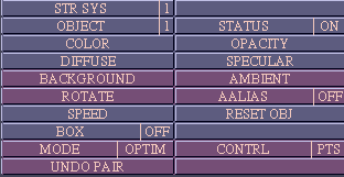
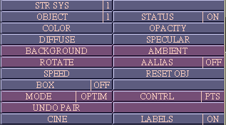
The panel options available for this command are shown in Figure 12.10.
A majority of the options function as described under VISUALIZE-Surface.
Other options are described below.
MODE: This option is a switch with three states called OPTIM, ALL PTS,
and SURF. In state ALL PTS, the specified points and the points sampled
on the specified curves are all optimally matched between the two
objects to arrive at the transformation needed for registration. In
state OPTIM, the points specified and the points sampled on specified
curves are checked for pairwise consistency. Those pairs that are most
inconsistent are deleted and not included in matching. Often this mode
leads to more accurate registration than ALL PTS. In state SURF, the
entire structures specified are optimally matched to determine the
needed transformation.
The default state of this switch is OPTIM.
UNDO PAIR: This is a button which when selected removes one pair of most
recently specified features -- points or curve.
CONTRL: This a switch with two states -- PTS and CRV. The switch should
be set to the appropriate value for specifying the desired control
features, points or curves, respectively.
Once registration is completed, to save the resulting plan, the SAVE
option in the mouse window should be selected after changing the output
file name if desired.
If you use control features for registration, it is generally a good
idea, for more accurate results, to select the features more
isotropically over the structure surface than concentrated on one side,
view, or area. You may want to register an object with itself for
getting an understanding of how features may be selected for best
results before you take on the actual registration task.
The plan files output by Register can be visualized (and measured) using
the VISUALIZE-Surface commands. To carry out further operations on
scenes that gave rise to the matched structures, you need to first
convert the plan output by Register into a plan containing Shell0
structures (via PREPROCESS-StructureOperation-Shell1ToShell0) and then
use this as input to MANIPULATE-SelectSlice. You may use this command to
select slices from scenes corresponding to the registered objects
through identical planes passing through the objects, overlay these
slices for comparing them and interpreting the density distributions,
and even output new scenes that are registered. These scenes may be
further input to ANALYZE-ROIStatistics or ANALYZE-DensityProfile for
further analysis of the cell density values in a comparative and
composite fashion.
Structure-Kinematics-Inter
The main purpose of this command is to compute and output as a plan the
motion of rigid objects captured in a set of input structure systems or
plans. It accepts two or more input files, each containing a structure
system or a plan or structures of type Shell1. Motion of a particular
object is determined by following the object with the same number in the
different input files, which are assumed to be the different instances
of the same object, computing the motion from the first to the second
instance, second to the third, and so on. Motion from instance t to the
next instance t+1 is expressed as a translation of the centroid of the
object, together with an axis of rotation, called instantaneous axis,
that passes through the centroid and an angle of rotation about this
axis. This motion takes the object from instance t to instance t+1. The
rotation and translation components are together expressed as a
transformation matrix that is associated with instance t of the object.
This becomes a part of the plan that is output. This command allows
creation of more instances than the number of instances represented in
the input files. This helps in smooth animation of kinematics.
To make these principles concrete, let us consider an example. Suppose
we have 2 objects whose rigid body motion is captured in 3 time
instances. That is, for each of the two objects, we have three
structures each of which represents a particular pose of the object
during its motion. (Such information may have come from a scanner. The
two objects may represent two bones of a moving joint and the three
instances may correspond to the three different positions of the joint
for each of which we acquired 3D image data.) The three time instances
are captured in three input files called, say, 1.BS1, 2.BS1, 3.BS1, each
of which contains two Shell1 structures which correspond to the two
objects at that particular time instance. We may represent the structure
systems contained in the three files as trees as shown in Figure
12.11(a). Suppose we wish to create 5 time instances for the output
plan. Then the tree representation of the output plan will be as in
Figure 12.11(b). The output plan actually does not store any structure
(Shell1) information. The nodes at the level indicated "objects" contain
pointers to the file 1.BS1 which contains the first instance of the two
objects. This is sufficient since the structures contained in other
files are different manifestations of the same two objects. These nodes
also have transformation matrices associated with them which indicate
their correct orientation at any time instance.
The order of time instances is taken to be in the alphabetical order of
the name of the input files. Therefore, the files should be named
appropriately when the structures are created for the different time
instances.
When this command is selected, kinematics computation is completed for
all objects in the input files and the results are reported as follow:
The panel options, shown in Figure 12.12, can be used to examine these
results object-by-object or as motion relative to some fixed object.
SCRL UP, SCRL DOWN: These are both buttons which allow scrolling up and
down the result displayed in the image window. This becomes necessary
when the input files contain several time instances.
OBJECT: This is a switch whose value indicates the number of the object
for which motion information is to be displayed.
REL TO: This is a switch which indicates the object relative to which
motion is to be determined. The default setting is NONE. This means that
motion of the objects computed and output is their absolute motion. For
other states, motion is computed relative to the object indicated. This
means that, when the output plan is displayed via VISUALIZE-Surface, the
object relative to which motion is computed will appear stationary and
other motions are relative to this apparently stationary object.
This command provides a scale labelled INSTANCES in the dialog window
for selecting the desired number of instances for the output. The
default setting on this scale is the number of instances in the input
files. The actual output operation of creating a PLN file is initiated
when the SAVE option in the output section of the mouse window is
selected. The nature of the motion information saved depends on the
state of the switch REL TO at the time of this operation.
There are other uses for this command than computing kinematics
information. We encourage the users to explore these on their own. For
example, it can be used to "interpolate" plans or for animating actions
based on plans. Suppose we create two plans or structure systems (via
MANIPULATE-Move), the first consisting of two objects which constitute
two separate segments of an original object (which are obtained via one
of the commands under MANIPULATE), and the second consisting of the same
two objects except that one of the objects is moved relative to the
other. If we input these into Kinematics-Inter and create an output with
sufficiently large number of instances, we will have created a smooth
animation of the movement of the moved object.
Structure-Kinematics-Intra
The purpose of this command is similar to that of Kinematics-Inter. The
only difference is that it accepts one input file containing a structure
system or a plan and it outputs a plan containing motion information
derived from the input file. Consider again the example given under
Kinematics-Inter (Figure 12.11). In order to compute the motion of the
two objects, we should build a structure system (via one of the commands
under SceneOperations) consisting of all time instances of all objects
as illustrated in Figure 12.13. Motion computation then proceeds exactly
as in Kinematics-Inter.
12.1.3.3 ROIStatistics
The main purpose of this command is to make it possible to compute ROI
statistics for regions-of-interest (rois) of certain fixed shape and
size and for user-drawn arbitrary regions. The statistics include:
minimum, maximum, mean, and standard deviation of cell density, and
minimum, maximum, mean, and standard deviation of gradient magnitude,
and area or volume of the region. Effectively, the user can sample
various regions within the scene domain, accumulate these statistics,
and save them in a file. As in the case of density profile, for dynamic
(4D) scenes, this command can be utilized to determine how the
statistics within fixed object regions change with time. Obviously, this
command can also be used to determine object area/volume or their change
with time for dynamic situations.
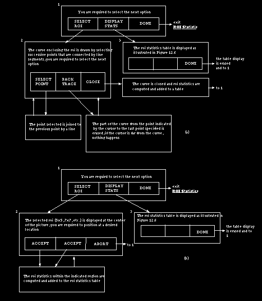
Fig 12.5: State Diagrams for ROIStatistics. An arrow leaving a button
indicates that that button is clicked. (a) For the case when the roi is
user-drawn (FREE), (b) for the case when the roi
is of predetermined size (e.g., 55, 77, 555, etc.).
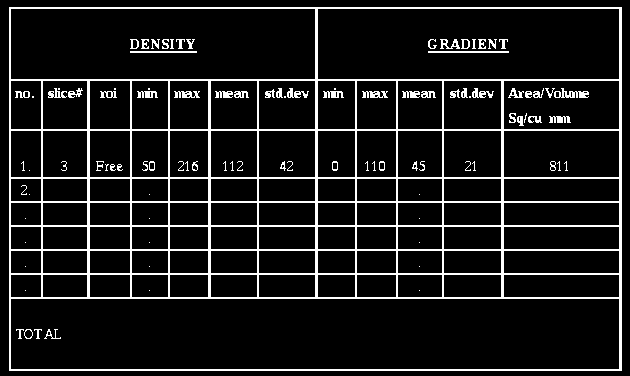
Fig 12.6: Format of the roi Statistics Table.
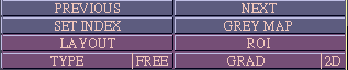
Fig 12.7: Panel Options for ROIStatistics.
12.2 Structure
12.2.1 Summary of Commands
The main purpose of these commands is advanced analysis of structures
and the structure systems.
12.2.2 Commands
12.2.2.1 Structure-Input
This command should be used to select the desired BS1 and PLN files. If
the most recently selected files are appropriate, it is not necessary to
initiate this command. For details of operation see Section 7.1.
12.2.2.2 Structure-Register
This command allows combining information about an object of study
obtained from two sources, for example, brain information from MR and
PET. Common structures, or structures containing common features about
the object of study, should be provided as input for each of the two
sources of information. It accepts two input files, each containing a
structure system or a plan, or just one input file containing a
structure system or plan, in each case of structures of type Shell1.
Corresponding structures in the input file(s) or corresponding features
of structures in the input file(s) are specified by the user. The
features used at present are points and curves. Registration is done by
optimally matching the two entire structures or the features specified
for them. The result of this operation is a structure plan. In the case
of one input file, the structure plan consists of the structures in the
input file (actually only pointers to them) together with a geometric
transformation matrix associated with each structure that represents the
translation and rotation required for two specified structures or
features on them to be optimally matched. In the case two input files,
the plan consists of only structures from the first input file together
with the transformation matrix. These are best explained with two
examples.
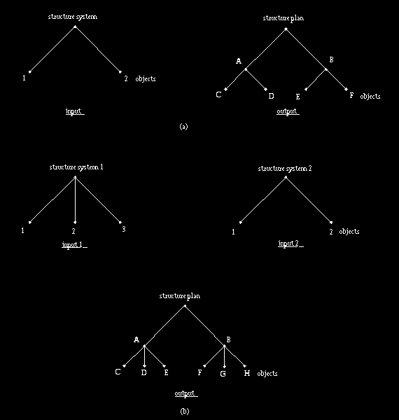
Fig 12.8: Examples used for illustrating Registration. (a) The case of one
input file, (b) the case of two input files.
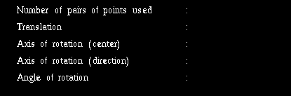
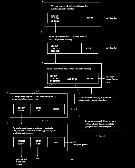
Fig 12.9a: State Diagram for Structure-Register. An arrow leaving a mouse
button area indicates that that button is clicked. Control features are points.
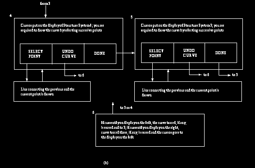
Fig 12.9b: State Diagram for Structure-Register. An arrow leaving a mouse
button area indicates that that button is clicked. Control features are curves
(up to state 3, same as in (a)).
 (a)
(a)
 (b)
(b)
Fig 12.10: Panel Options for Structure-Register. (a) When the number of
elements in the parameter vector is 1. (b) When this number is greater
than 1.
12.2.2.3 Structure-Kinematics
Kinematics has two commands under it called Inter and Intra.
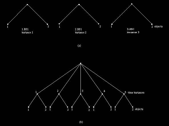
Fig 12.11: An Example to Illustrate how Kinematics-Inter works. (a) Input,
(b) Output.
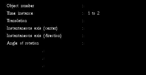

Fig 12.12: Panel Options for Kinematics-Inter.
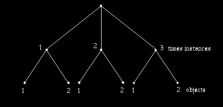
Fig 12.13: A structure system consisting of 3 time instances for each of 2
objects. It contains the same information as contained in the three files
illustrated in Figure 12.11a.
 User Manual
 Library Ref. Manual
 Tutorial